
Spatial analysis
In the field of my study, many datasets contain the information of the location, and these information will impact the results of the analyses. Moreover, we will always acquire new knowledge from these spatial data. For the location-based data, specific analytical techniques will be used. Here I list some very very basic functions in R for spatial analysis. I suggest two books Applied Spatial Data Analysis with R and An Introduction to R for Spatial Analysis and Mapping for further reading.
Datasets from the web for this post
- Population and Location of US State Capitals from 2010 census “us-capitals.csv”
- Cartographic Boundary Shapefiles (Counties) of USA from 2010 census at 1:20,000,000 scale “gz_2010_us_050_00_20m.shp”
- Global altitude at 10 arc-minute resolution “alt.bil”
- American National Standards Institute (ANSI) Codes for States “state.txt”
I use these datasets to demonstrate some useful (but limited) functions for spatial analysis, not for any special purpose here. There are some other useful tutorials (this, this, this and this)
Import data
1
2
3
4
5
6
7
8
9
10
11
12
13
14
15
16
17
18
19
20
21
22
23
24
25
26
27
28
29
30
31
32
33
34
35
36
37
38
39
40
41
42
43
44
45
46
47
48
49
50
51
52
53
54
55
56
57
58
59
60
61
62
63
64
65


# Import points from data frame
library(sp)
library(rgdal)
library(raster)

capital <- read.csv("us-capitals.csv")
class(capital)
## [1] "data.frame"

head(capital)
##   id abbrev      state     capital latitude  longitude population
## 1  1     AL    Alabama  Montgomery 32.38012  -86.30063     205764
## 2  2     AK     Alaska      Juneau 58.29974 -134.40679      31275
## 3  4     AZ    Arizona     Phoenix 33.44826 -112.07577    1445632
## 4  5     AR   Arkansas Little Rock 34.74865  -92.27449     193524
## 5  6     CA California  Sacramento 38.57906 -121.49101     466488
## 6  8     CO   Colorado      Denver 39.74001 -104.99226     600158

# Create a SpatialPointsDataFrame
coordinates(capital) <- ~longitude+latitude

capital
## class       : SpatialPointsDataFrame
## features    : 50
## extent      : -157.8576, -69.77622, 21.30477, 58.29974  (xmin, xmax, ymin, ymax)
## coord. ref. : NA
## variables   : 5
## names       : id, abbrev,   state, capital, population
## min values  :  1,     AK, Alabama,  Albany,       7855
## max values  : 56,     WY, Wyoming, Trenton,    1445632

# Set the projection attributes, it seems to be WGS84
proj4string(capital) <- CRS("+proj=longlat
    +datum=WGS84 +no_defs
    +ellps=WGS84 +towgs84=0,0,0") # PROJ.4 projection system
                                  # (https://github.com/OSGeo/proj.4)

# Read polygons (shapefiles)
poly <- readOGR(
            dsn=".",                      # data source name
            layer="gz_2010_us_050_00_20m" # layer name
                )

poly
## class       : SpatialPolygonsDataFrame
## features    : 3221
## extent      : -179.1473, 179.7785, 17.88481, 71.35256  (xmin, xmax, ymin, ymax)
## coord. ref. : +proj=longlat +datum=NAD83 +no_defs +ellps=GRS80 +towgs84=0,0,0
## variables   : 6
## names       :         GEO_ID, STATE, COUNTY,     NAME,    LSAD, CENSUSAREA
## min values  : 0500000US01001,    01,    001, Accomack, Borough,      1.999
## max values  : 0500000US72153,    72,    840,  Ziebach,  Parish, 145504.789

# Load raster data
alt <- raster("alt.bil") # see help file for more information

alt
## class       : RasterLayer
## dimensions  : 900, 2160, 1944000  (nrow, ncol, ncell)
## resolution  : 0.1666667, 0.1666667  (x, y)
## extent      : -180, 180, -60, 90  (xmin, xmax, ymin, ymax)
## coord. ref. : +proj=longlat +ellps=WGS84 +towgs84=0,0,0,0,0,0,0 +no_defs
## data source : H:alt.bil
## names       : alt
## values      : -353, 6241  (min, max)
Union
1
2
3
4
5
6
7
8
9
10
11
12
13
14
15
16
17
18
19
20
21
22
23
24
25
26
27
28
29
30
31
32
33
34
35
36
37
38
39
40
41
42
43
44
45
46
47
48
49
50
51
52
53
54
55
56
57
58
59
60
61
62
63


library(maptools)
# 1. Aggregate counties to states
polyU <- unionSpatialPolygons(
            poly,                   # a SpatialPolygons object
            IDs=poly@data[,"STATE"] # a vector defining the
                                    # output Polygons objects
            )

polyU
## class       : SpatialPolygons
## features    : 52
## extent      : -179.1473, 179.7785, 17.88481, 71.35256  (xmin, xmax, ymin, ymax)
## coord. ref. : +proj=longlat +datum=NAD83 +no_defs +ellps=GRS80 +towgs84=0,0,0

# 2. Transform SpatialPolygons to SpatialPolygonsDataFrame

# State's code in the SpatialPolygonsDataFrame,
# add a new attribute, number of counties in each state
states <- stats::aggregate(poly@data[,"STATE"],
        list(poly@data[,"STATE"]),length)

names(states) <- c("state_code","num")

head(states)
##   state_code num
## 1         01  67
## 2         02  29
## 3         04  15
## 4         05  75
## 5         06  58
## 6         08  64

# Read codes for states, then merge "states" with state names
stateName <- read.table("state.txt",sep="|",
                header=T,colClasses="factor")
states <- base::merge(states,stateName,
                by.x="state_code",by.y="STATE",all.x=T)
rownames(states) <- states[,"state_code"]

head(states)
##    state_code num STUSAB STATE_NAME  STATENS
## 01         01  67     AL    Alabama 01779775
## 02         02  29     AK     Alaska 01785533
## 04         04  15     AZ    Arizona 01779777
## 05         05  75     AR   Arkansas 00068085
## 06         06  58     CA California 01779778
## 08         08  64     CO   Colorado 01779779

# New dissolved SpatialPolygonsDataFrame
polyUD <- SpatialPolygonsDataFrame(
            polyU, # SpatialPolygons
            states # data frame with attributes
            )

polyUD
## class       : SpatialPolygonsDataFrame
## features    : 52
## extent      : -179.1473, 179.7785, 17.88481, 71.35256  (xmin, xmax, ymin, ymax)
## coord. ref. : +proj=longlat +datum=NAD83 +no_defs +ellps=GRS80 +towgs84=0,0,0
## variables   : 5
## names       : state_code, num, STUSAB, STATE_NAME,  STATENS
## min values  :         01,   1,     AK,    Alabama, 00068085
## max values  :         72, 254,     WY,    Wyoming, 01785534
Projection
When we manipulate the spatial data with different coordinate reference systems (CRS), it is important to transform their projections to the same CRS first. I transform the spatial points and raster to the CRS of the polygons here.
1
2
3
4
5
6
7
8
9
10
11
12
13
14
15
16
17
18
19
20
21
22
23
24
25
26
27
28
29
30
31
32
33
34
35
36
37
38
39
40
41


projection(capital)
## [1] "+proj=longlat +datum=WGS84 +no_defs +ellps=WGS84 +towgs84=0,0,0"

projection(polyUD)
## [1] "+proj=longlat +datum=NAD83 +no_defs +ellps=GRS80 +towgs84=0,0,0"

projection(alt)
## [1] "+proj=longlat +ellps=WGS84 +towgs84=0,0,0,0,0,0,0 +no_defs"

# Project a Spatial object
capital <- spTransform(         # see help file for more information
        capital,                # Spatial* object
        CRS(projection(polyUD)) # coordinate reference system
        )

capital
## class       : SpatialPointsDataFrame
## features    : 50
## extent      : -157.8576, -69.77622, 21.30477, 58.29974  (xmin, xmax, ymin, ymax)
## coord. ref. : +proj=longlat +datum=NAD83 +no_defs +ellps=GRS80 +towgs84=0,0,0
## variables   : 5
## names       : id, abbrev,   state, capital, population
## min values  :  1,     AK, Alabama,  Albany,       7855
## max values  : 56,     WY, Wyoming, Trenton,    1445632

# Project a Raster object
alt <- projectRaster(                # see help file for more information
        alt,                         # Raster* object
        crs=CRS(projection(polyUD)), # coordinate reference system
        method="bilinear"            # method for computing new values
        )

alt
## class       : RasterLayer
## dimensions  : 903, 2156, 1946868  (nrow, ncol, ncell)
## resolution  : 0.167, 0.167  (x, y)
## extent      : -180, 180.052, -60.801, 90  (xmin, xmax, ymin, ymax)
## coord. ref. : +proj=longlat +datum=NAD83 +no_defs +ellps=GRS80 +towgs84=0,0,0
## data source : in memory
## names       : alt
## values      : -148.8531, 5980.991  (min, max)
Clip
1
2
3
4
5
6
7
8
9
10
11
12
13
14
15
16
17
18
19
20
21
22
23
24
25
26
27
28
29
30
31
32
33
34
35
36
37
38
39
40
41
42
43
44
45
46


# I will focus the mainland of USA,
# so exclude the non-contiguous areas
mainland <- polyUD[!(polyUD$STATE_NAME %in%
        c("Alaska","Hawaii","Puerto Rico","Rhode Island")),]

# Plot, see Fig. 1
par(mfrow=c(1,2))
plot(polyUD,main="Entire United States")
box()
plot(mainland,main="Contiguous United States")
box()
par(mfrow=c(1,1))

# The capitals in mainland
capitcalMain <- intersect(capital, mainland)

capitcalMain # there is no capital for District of Columbia
## class       : SpatialPointsDataFrame
## features    : 47
## extent      : -123.0438, -69.77622, 30.26761, 47.03923  (xmin, xmax, ymin, ymax)
## coord. ref. : +proj=longlat +datum=NAD83 +no_defs +ellps=GRS80 +towgs84=0,0,0
## variables   : 10
## names       : id, abbrev,   state, capital, population, state_code, num, STUSAB, STATE_NAME,  STATENS
## min values  :  1,     AL, Alabama,  Albany,       7855,         01,   3,     AL,    Alabama, 00068085
## max values  : 56,     WY, Wyoming, Trenton,    1445632,         56, 254,     WY,    Wyoming, 01785534

# Crop a geographic subset from the raster
# "alt" by an "extent" object
altCrop <- crop(alt, mainland)

# Mask values in a Raster object
altMask <- mask(       # see help file for more information
        x=altCrop,     # Raster* object
        mask=mainland, # Spatial* object here
        inverse=FALSE, # mask which area on the "mask"
                       # object (NA cells or not NA cells)
        updatevalue=NA # value for the cells that are not covered by the "mask"
)

# The "altCrop" and "altMask" are different, see Fig. 2
par(mfrow=c(1,2))
plot(altCrop,axes=F,box=F,legend=F,main="Cropped")
box()
plot(altMask,axes=F,box=F,legend=F,main="Masked")
box()
par(mfrow=c(1,1))
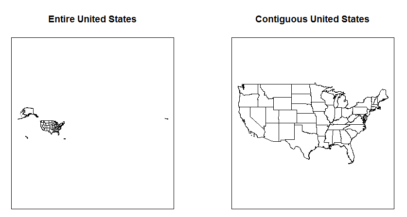
Figure 1 Map of United States.
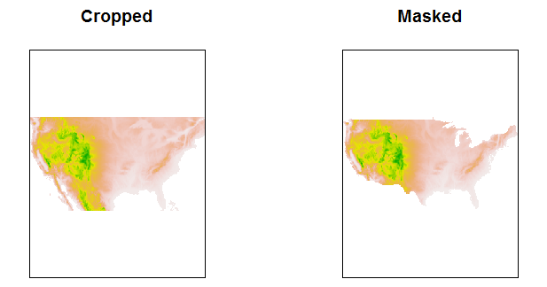
Figure 2 Cropped and masked raster.
Extract values
1
2
3
4
5
6
7
8
9
10
11
12
13
14
15
16
17
18
19
20
21
22
23
24
25
26
27
28
29
30
31
32
33
34
35
36
37
38
39
40
41
42
43
44


# Altitude of the capitals
capitalAlt <- extract(alt, capital) # see help file for more information

capitalAlt
##  [1]   72.24102  714.84681  361.96860   99.47084   14.10031 1609.28407
##  [7]   62.40934   11.39256   41.78794  291.73066   84.30727 1241.34990
## [13]  175.18235  241.23507  267.24544  313.87901  234.83596   13.26608
## [19]   69.31159   22.20674   28.31122  268.98132  269.81409  100.25913
## [25]  217.31235 1266.21281  377.30116 1739.26864  146.75366   26.58871
## [31] 2172.69415  103.95782  116.49673  543.81899  253.09422  375.62256
## [37]   83.88169  163.72515   70.14791   77.77868  516.92393  176.59067
## [43]  206.98887 1369.33335  387.47802   41.70075   90.48425  280.99556
## [49]  285.77906 1862.65204

# Maximum altitude of each state
stateAlt <- extract(
        alt,      # Raster* object
        mainland, # SpatialPolygons* object
        df=TRUE,  # results as a data.frame
        fun=max   # function to summarize the values
        )

head(cbind(state=as.character(mainland$STATE_NAME),stateAlt))
##         state ID       alt
## 1     Alabama  1  426.1076
## 2     Arizona  2 2833.4440
## 3    Arkansas  3  572.2969
## 4  California  4 3246.8690
## 5    Colorado  5 3563.2026
## 6 Connecticut  6  377.6199

# Sometimes it will be quite useful if we have
# the coordinates of the center of raster cells
index <- cellFromXY(alt, capital)
captialGrid <- xyFromCell(alt, index)

head(captialGrid)
##              x       y
## [1,]  -86.2295 32.3015
## [2,] -134.3255 58.3535
## [3,] -112.1145 33.4705
## [4,]  -92.2415 34.8065
## [5,] -121.4665 38.6475
## [6,] -104.9335 39.8165
Resample
1
2
3
4
5
6
7
8
9
10
11
12
13
14
15
16
17
18
19
20
21
22
23
24
25
26
27
28
29
30
31
32
33
34
35


# Aggregate from 10 arc-minute to 30 arc-minute
alt30 <- aggregate(
        alt,        # Raster* object
        fact=3,     # aggregation factor
        fun=mean    # function used to aggregate values
        )

alt30
## class       : RasterLayer
## dimensions  : 301, 719, 216419  (nrow, ncol, ncell)
## resolution  : 0.501, 0.501  (x, y)
## extent      : -180, 180.219, -60.801, 90  (xmin, xmax, ymin, ymax)
## coord. ref. : +proj=longlat +datum=NAD83 +no_defs +ellps=GRS80 +towgs84=0,0,0
## data source : in memory
## names       : alt
## values      : -74.12883, 5607.752  (min, max)

# Resample a raster
resampleTo <- raster(nrow=100,ncol=100) # define a new raster

altRe <- resample(
        alt,              # Raster* object to be resampled
        resampleTo,       # Raster* object that "x" should be resampled to
        method="bilinear" # method used to compute values
        )

altRe
## class       : RasterLayer
## dimensions  : 100, 100, 10000  (nrow, ncol, ncell)
## resolution  : 3.6, 1.8  (x, y)
## extent      : -180, 180, -90, 90  (xmin, xmax, ymin, ymax)
## coord. ref. : +proj=longlat +datum=WGS84 +ellps=WGS84 +towgs84=0,0,0
## data source : in memory
## names       : alt
## values      : -24.3118, 5260.449  (min, max)
Plot
1
2
3
4
5
6
7
8
9
10
11
12
13
14
15
16
17
18
19
20
21
22
23
24
25
26
27
28
29
30
31
32
33
34
35
36
37
38
39
40
41
42
43
44
45
46
47
48
49
50


# Plot altitude of contiguous USA
plot(
    altMask,                      # Raster* object
    col=rev(terrain.colors(255)), # colors
    colNA="#5F9EA0",              # color for the background
    axes=FALSE,                   # no axes
    box=FALSE,                    # no box
    legend=FALSE,                 # no legend
   )

# Add legend, see http://stackoverflow.com/questions/9436947/legend-properties-when-legend-only-t-raster-package
# for legend setting
plot(
    altMask,                                # Raster* object
    legend.only=TRUE,                       # legend only
    col=rev(terrain.colors(255)),           # color for legend
    axis.args=list(at=seq(0,3000,1000),     # axis setting
                labels=seq(0,3,1)),
    legend.args=list(text='Altitude (km)',  # legend setting
                side=4,line=1.5,font=2)
    )

# Add polygons
plot(
    mainland,          # a SpatialPolygons object
    col="transparent", # fill color
    border="white",    # color of border
    lwd=2,             # border line width
    add=TRUE           # add to existing plot
    )

# Add state names
text(mainland,              # SpatialPolygons* object
    labels=mainland$STUSAB, # labels
    font=2,                 # font
    col="black",            # color
    cex=0.7                 # label size
    )

# Add captials
plot(
    capitcalMain,                        # SpatialPoints object
    pch=21,                              # symbol
    add=TRUE,                            # add to existing plot
    cex=(capitcalMain$population)
        /max(capitcalMain$population)*5, # size of the points
    col="red",                           # color
    bg="transparent",                    # background color
    lwd=2                                # line width
    )
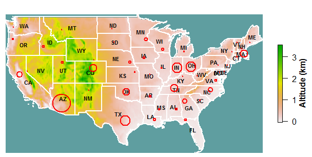
Figure 3 Altitude and population of contiguous USA.
There are just few frequently-used functions, do more explorations for complicated and practical functions.


近期评论