
When the anomaly data is very few, we need to make good use of F1 Score to help us to figure out which model is better.
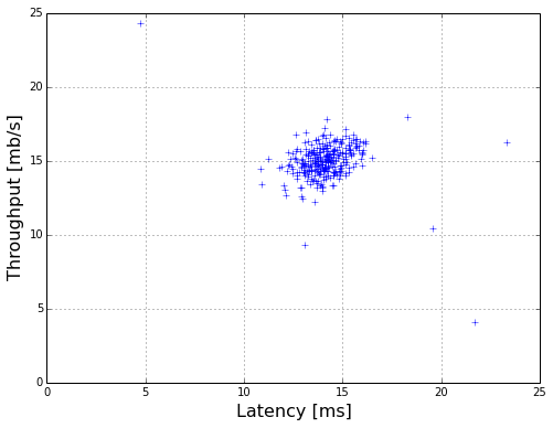
plot the data
    # import modules
    %matplotlib inline
    import numpy as np
    import matplotlib.pyplot as plt
    import scipy.io # used to load the mat files
    import scipy.optimize

    # load the data into numpy
    filename = 'ex8/data/ex8data1.mat'
    mat = scipy.io.loadmat(filename)
    print mat['X'].shape,mat['Xval'].shape,mat['yval'].shape
(307, 2) (307, 2) (307, 1)
    X = mat['X']
    Xval = mat['Xval']
    yval = mat['yval']

    def plotData(myX, newFig = True):
        if newFig:
            plt.figure(figsize=(8,6))
        plt.plot(myX[:,0],myX[:,1],'b+')
        plt.xlabel('Latency [ms]',fontsize=16)
        plt.ylabel('Throughput [mb/s]',fontsize=16)
        plt.grid(True)
        plt.show()

    plotData(X)
cal the mean and deviration
    def estimateGaussian(myX):
        """
        compute the mean and deviration of the array-like:myX, then return the mean and deviration
        """
        mu = np.mean(myX,axis=0)
        deviration = myX - mu
        dev2 = np.sum(np.power(deviration,2),axis=0)
        return mu,dev2 / myX.shape[0]

    mu,dev2 = estimateGaussian(X)
    print mu.shape, dev2
(2,) [ 1.83263141 1.70974533]
cal the probability
print np.diag(dev2),np.linalg.det(np.diag(dev2))
the output is:
    [[ 1.83263141  0.        ]
     [ 0.          1.70974533]]
    3.13333300235
    def gaus(myX, mymu, mysig2):
        """
        Function to compute the gaussian return values for a feature,
        matrix, myX, given the already computed mu vector and sigma matrix.,
        If sigma is a vector, it is turned into a diagonal matrix,
        Uses a loop over rows; I didn't quite figure out a vectorized implementation.
        """
        m = myX.shape[0]
        n = myX.shape[1]

        if np.ndim(mysig2) == 1:
            mysig2 = np.diag(mysig2)

        norm = 1.0 / (np.power(2.0 * np.pi, n /2.0) * np.sqrt(np.linalg.det(mysig2)))
        myinv = np.linalg.inv(mysig2)
        myexp = np.zeros((m,1))
        for irow in xrange(m):
            xrow= myX[irow]
            myexp[irow] = np.exp(-0.5*((xrow-mymu).T).dot(myinv).dot(xrow-mymu))
        return norm * myexp

    p = gaus(X,mu,dev2)

    print p[:10]
the output is:
    [[ 0.06470829]
     [ 0.05030417]
     [ 0.07245035]
     [ 0.05031575]
     [ 0.06368497]
     [ 0.04245832]
     [ 0.04790945]
     [ 0.03651115]
     [ 0.0186658 ]
     [ 0.05068826]]
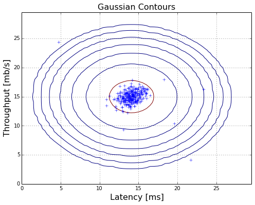
contour the gaussian distribution
    def plotContours(myX, mymu, mysigma2, newFig=False, useMultivariate = True):
        delta = 0.5
        myx = np.arange(0,30,delta)
        myy = np.arange(0,30,delta)

        meshx,meshy = np.meshgrid(myx,myy)

        coord_list = [ entry.ravel() for entry in (meshx, meshy) ]

        points = np.vstack(coord_list)
        myz = gaus(points.T,mymu,mysigma2)

        #print myz[:,0].shape
        myz = myz.reshape((myx.shape[0],myx.shape[0]))
        if newFig:
            plt.figure(figsize=(8,6))
        plt.plot(myX[:,0],myX[:,1],'b+')
        plt.xlabel('Latency [ms]',fontsize=16)
        plt.ylabel('Throughput [mb/s]',fontsize=16)
        plt.grid(True)
        cont_levels = [10**exp for exp in range(-20,0,3)]
        mycont = plt.contour(meshx,meshy,myz,cont_levels)
        plt.title('Gaussian Contours',fontsize=16)

    plotContours(X,mu,dev2,True,True)
    #plt.show()
F1 score
implementation
    def selectThreshold(yval,pval):
        """
        yval:label
        pval:predict value
        function: according to both yval and pval to cal the F1 Score
        """
        yval = yval.flatten()
        pval = pval.flatten()
        bestEpis = 0.0
        bestF1 = 0.0
        m = len(yval)
        step = (np.max(pval) - np.min(pval)) / float(1000)
        minv = np.min(pval)

        for v in xrange(1000):
            episode = minv + v * step
            tp = np.sum(np.bitwise_and(pval < episode, yval==1))
            fp = np.sum(np.bitwise_and(pval < episode, yval==0))
            fn = np.sum(np.bitwise_and(pval > episode, yval==1))
            #print tp,fp,fn
            if tp + fp ==0:
                continue
            pre = float(tp)/(tp + fp)
            if tp + fn == 0:
                continue
            rec = float(tp)/(tp + fn)
            if (pre + rec)==0:
                continue
            F1 = 2 * pre * rec/(pre + rec)
            if F1 > bestF1:
                bestF1 = F1
                bestEpis = episode
        return bestF1, bestEpis

    pval = gaus(Xval,mu,dev2)
    bestF1, bestEpis = selectThreshold(yval,pval)
    print "best F1 score is:%s,and best episode is:%s)" % ( bestF1, bestEpis )
best F1 score is:0.875,and best episode is:8.99085277927e-05)
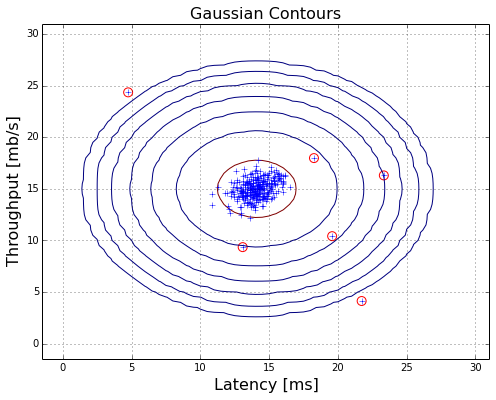
visualization
    def plotAnomalies(myX,mybestEps, newFig = False):
        ps = gaus(myX,*estimateGaussian(myX))
        ps = ps.flatten()
        anoms = myX[ps < mybestEps]
        if newFig:
            plt.figure(figsize=(6,4))
        plt.scatter(anoms[:,0],anoms[:,1],s=80,facecolors='none',edgecolors='r')

    plotContours(X,mu,dev2,True,True)
    plotAnomalies(X,bestEpis,False)
    #plt.show()
test on 11 dimension samples
    filename = 'ex8/data/ex8data2.mat'
    mat = scipy.io.loadmat(filename)
    X=mat['X']
    Xval = mat['Xval']
    yval = mat['yval']
    print X.shape,Xval.shape,yval.shape
(1000, 11) (100, 11) (100, 1)
    mu,sigma2 = estimateGaussian(X)
    p = gaus(X,mu,sigma2)
    pval = gaus(Xval,mu,sigma2)
    bestF1, bestEpis = selectThreshold(yval,pval)

    print 'Best epsilon found using cross-validation:%s', bestEpis
    print 'Best F1 found on cross validation set: %s', bestF1
    print '#Outliers found: %d' % np.sum(p < bestEpis)
Best epsilon found using cross-validation:%s 1.37722889076e-18
Best F1 found on cross validation set: %s 0.615384615385
#Outliers found: 117


近期评论