%matplotlib inline
    import os
    import pandas as pd
    import numpy as np

    def symbol_to_path(symbol, base_dir="stock/data"):
        """Return CSV file path given ticker symbol."""
        return os.path.join(base_dir, "{}.csv".format(str(symbol)))

    def get_data(symbols, dates):
        """Read stock data (adjusted close) for given symbols from CSV files."""
        df = pd.DataFrame(index=dates)
        if 'SPY' not in symbols:  # add SPY for reference, if absent
            symbols.insert(0, 'SPY')

        for symbol in symbols:
            # TODO: Read and join data for each symbol
            df1 = pd.read_csv(symbol_to_path(symbol),index_col='Date', usecols=['Date','Adj Close'],parse_dates=True,na_values=['nan'])
            df1=df1.rename(columns={'Adj Close':symbol})
            df = df.join(df1)
            if symbol=='SPY':
                df=df.dropna()
        return df

    def test_run1():
        # Define a date range
        dates = pd.date_range('2010-01-01', '2010-01-10')

        # Choose stock symbols to read
        symbols = ['GOOG', 'IBM', 'AAPL']

        # Get stock data
        df = get_data(symbols, dates)

        print df

        print "the mean value is:n%s" % df.mean()

        print "the medim value is:n %s" % df.median()

        print "the deviation value is:n %s n and sum is:n %s" % (df.std(), df.sum())

        return

    test_run()

                      SPY        GOOG         IBM       AAPL
    2010-01-04  98.793254  313.062468  112.285875  27.847252
    2010-01-05  99.054769  311.683844  110.929466  27.895396
    2010-01-06  99.124509  303.826685  110.208865  27.451683
    2010-01-07  99.542943  296.753749  109.827375  27.400936
    2010-01-08  99.874198  300.709808  110.929466  27.583106
    the mean value is:
    SPY      99.277935
    GOOG    305.207311
    IBM     110.836209
    AAPL     27.635675
    dtype: float64
    the medim value is:
     SPY      99.124509
    GOOG    303.826685
    IBM     110.929466
    AAPL     27.583106
    dtype: float64
    the deviation value is:
     SPY     0.428374
    GOOG    7.022203
    IBM     0.939446
    AAPL    0.225798
    dtype: float64 
     and sum is:
     SPY      496.389673
    GOOG    1526.036554
    IBM      554.181047
    AAPL     138.178373
    dtype: float64

    """Bollinger Bands."""

    import matplotlib.pyplot as plt

    def plot_data(df, title="Stock prices"):
        """Plot stock prices with a custom title and meaningful axis labels."""
        ax = df.plot(title=title, fontsize=12)
        ax.set_xlabel("Date")
        ax.set_ylabel("Price")
        plt.show()

    def get_rolling_mean(values, window):
        """Return rolling mean of given values, using specified window size."""
        return values.rolling( window=window).mean()

    def get_rolling_std(values, window):
        """Return rolling standard deviation of given values, using specified window size."""
        # TODO: Compute and return rolling standard deviation
        return values.rolling(window).std()

    def get_bollinger_bands(rm, rstd):
        """Return upper and lower Bollinger Bands."""
        # TODO: Compute upper_band and lower_band
        upper_band = rm + 2 * rstd
        lower_band = rm - 2 * rstd
        return upper_band, lower_band

    def test_run2():
        # Read data
        dates = pd.date_range('2012-01-01', '2012-12-31')
        symbols = ['SPY']
        df = get_data(symbols, dates)

        # Compute Bollinger Bands
        # 1. Compute rolling mean
        rm_SPY = get_rolling_mean(df['SPY'], window=20)

        # 2. Compute rolling standard deviation
        rstd_SPY = get_rolling_std(df['SPY'], window=20)

        # 3. Compute upper and lower bands
        upper_band, lower_band = get_bollinger_bands(rm_SPY, rstd_SPY)

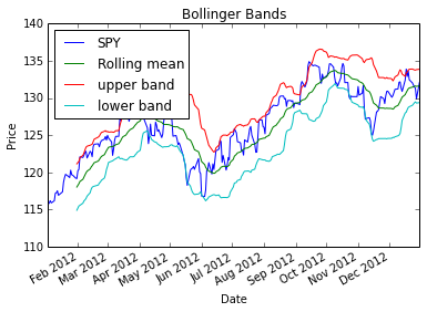
        # Plot raw SPY values, rolling mean and Bollinger Bands
        ax = df['SPY'].plot(title="Bollinger Bands", label='SPY')
        rm_SPY.plot(label='Rolling mean', ax=ax)
        upper_band.plot(label='upper band', ax=ax)
        lower_band.plot(label='lower band', ax=ax)

        # Add axis labels and legend
        ax.set_xlabel("Date")
        ax.set_ylabel("Price")
        ax.legend(loc='upper left')
        plt.show()

    test_run2()