
Pandas
Pandas is an open source, BSD-licensed library providing high-performance, easy-to-use data structures and data analysis tools for the Python programming language.
Library documentation: http://pandas.pydata.org/
General
In:
import numpy as np
import pandas as pd
import matplotlib.pyplot as plt
%matplotlib inline

# create a series
s = pd.Series([1,3,5,np.nan,6,8])
s
Out:
0     1
1     3
2     5
3   NaN
4     6
5     8
dtype: float64
In:
# create a data frame
dates = pd.date_range('20130101',periods=6)
df = pd.DataFrame(np.random.randn(6,4),index=dates,columns=list('ABCD'))
df
Out:
| A | B | C | D | |
|---|---|---|---|---|
| 2013-01-01 | 0.205240 | 0.527603 | 0.610052 | 0.469292 |
| 2013-01-02 | 0.818113 | -0.894390 | -1.602831 | 0.862170 |
| 2013-01-03 | -1.462109 | 0.483201 | -1.044973 | -0.534227 |
| 2013-01-04 | 0.719197 | -0.499809 | 1.145788 | -0.809526 |
| 2013-01-05 | -1.161051 | -0.115774 | -0.624413 | 0.474422 |
| 2013-01-06 | 0.000782 | 0.146544 | 0.033628 | -0.419772 |
In:
# another way to create a data frame
df2 = pd.DataFrame(
    { 'A' : 1.,
      'B' : pd.Timestamp('20130102'),
      'C' : pd.Series(1,index=list(range(4)),dtype='float32'),
      'D' : np.array([3] * 4,dtype='int32'),
      'E' : 'foo' })
df2
Out:
| A | B | C | D | E | |
|---|---|---|---|---|---|
| 0 | 1 | 2013-01-02 | 1 | 3 | foo |
| 1 | 1 | 2013-01-02 | 1 | 3 | foo |
| 2 | 1 | 2013-01-02 | 1 | 3 | foo |
| 3 | 1 | 2013-01-02 | 1 | 3 | foo |
In:
df2.dtypes
Out:
A           float64
B    datetime64[ns]
C           float32
D             int32
E            object
dtype: object
In:
df.head()
Out:
| A | B | C | D | |
|---|---|---|---|---|
| 2013-01-01 | 0.205240 | 0.527603 | 0.610052 | 0.469292 |
| 2013-01-02 | 0.818113 | -0.894390 | -1.602831 | 0.862170 |
| 2013-01-03 | -1.462109 | 0.483201 | -1.044973 | -0.534227 |
| 2013-01-04 | 0.719197 | -0.499809 | 1.145788 | -0.809526 |
| 2013-01-05 | -1.161051 | -0.115774 | -0.624413 | 0.474422 |
In:
df.index
Out:
<class 'pandas.tseries.index.DatetimeIndex'>
[2013-01-01, ..., 2013-01-06]
Length: 6, Freq: D, Timezone: None
In:
df.columns
Out:
Index([u'A', u'B', u'C', u'D'], dtype='object')
In:
df.values
Out:
array([[  2.05240362e-01,   5.27602841e-01,   6.10052272e-01,
          4.69292270e-01],
       [  8.18112883e-01,  -8.94389618e-01,  -1.60283098e+00,
          8.62169894e-01],
       [ -1.46210940e+00,   4.83201108e-01,  -1.04497297e+00,
         -5.34226832e-01],
       [  7.19196807e-01,  -4.99809344e-01,   1.14578824e+00,
         -8.09525609e-01],
       [ -1.16105080e+00,  -1.15774007e-01,  -6.24412514e-01,
          4.74421893e-01],
       [  7.82298420e-04,   1.46543576e-01,   3.36282758e-02,
         -4.19771560e-01]])
In:
# quick data summary
df.describe()
Out:
| A | B | C | D | |
|---|---|---|---|---|
| count | 6.000000 | 6.000000 | 6.000000 | 6.000000 |
| mean | -0.146638 | -0.058771 | -0.247125 | 0.007060 |
| std | 0.957650 | 0.561381 | 1.036400 | 0.679012 |
| min | -1.462109 | -0.894390 | -1.602831 | -0.809526 |
| 25% | -0.870593 | -0.403801 | -0.939833 | -0.505613 |
| 50% | 0.103011 | 0.015385 | -0.295392 | 0.024760 |
| 75% | 0.590708 | 0.399037 | 0.465946 | 0.473139 |
| max | 0.818113 | 0.527603 | 1.145788 | 0.862170 |
In:
df.T
Out:
| 2013-01-01 00:00:00 | 2013-01-02 00:00:00 | 2013-01-03 00:00:00 | 2013-01-04 00:00:00 | 2013-01-05 00:00:00 | 2013-01-06 00:00:00 | |
|---|---|---|---|---|---|---|
| A | 0.205240 | 0.818113 | -1.462109 | 0.719197 | -1.161051 | 0.000782 |
| B | 0.527603 | -0.894390 | 0.483201 | -0.499809 | -0.115774 | 0.146544 |
| C | 0.610052 | -1.602831 | -1.044973 | 1.145788 | -0.624413 | 0.033628 |
| D | 0.469292 | 0.862170 | -0.534227 | -0.809526 | 0.474422 | -0.419772 |
In:
# axis 0 is index, axis 1 is columns
df.sort_index(axis=1, ascending=False)
Out:
| D | C | B | A | |
|---|---|---|---|---|
| 2013-01-01 | 0.469292 | 0.610052 | 0.527603 | 0.205240 |
| 2013-01-02 | 0.862170 | -1.602831 | -0.894390 | 0.818113 |
| 2013-01-03 | -0.534227 | -1.044973 | 0.483201 | -1.462109 |
| 2013-01-04 | -0.809526 | 1.145788 | -0.499809 | 0.719197 |
| 2013-01-05 | 0.474422 | -0.624413 | -0.115774 | -1.161051 |
| 2013-01-06 | -0.419772 | 0.033628 | 0.146544 | 0.000782 |
In:
# can sort by values too
df.sort(columns='B')
Out:
| A | B | C | D | |
|---|---|---|---|---|
| 2013-01-02 | 0.818113 | -0.894390 | -1.602831 | 0.862170 |
| 2013-01-04 | 0.719197 | -0.499809 | 1.145788 | -0.809526 |
| 2013-01-05 | -1.161051 | -0.115774 | -0.624413 | 0.474422 |
| 2013-01-06 | 0.000782 | 0.146544 | 0.033628 | -0.419772 |
| 2013-01-03 | -1.462109 | 0.483201 | -1.044973 | -0.534227 |
| 2013-01-01 | 0.205240 | 0.527603 | 0.610052 | 0.469292 |
Selection
In:
# select a column (yields a series)
df['A']
Out:
2013-01-01    0.205240
2013-01-02    0.818113
2013-01-03   -1.462109
2013-01-04    0.719197
2013-01-05   -1.161051
2013-01-06    0.000782
Freq: D, Name: A, dtype: float64
In:
# column names also attached to the object
df.A
Out:
2013-01-01    0.205240
2013-01-02    0.818113
2013-01-03   -1.462109
2013-01-04    0.719197
2013-01-05   -1.161051
2013-01-06    0.000782
Freq: D, Name: A, dtype: float64
In:
# slicing works
df[0:3]
Out:
| A | B | C | D | |
|---|---|---|---|---|
| 2013-01-01 | 0.205240 | 0.527603 | 0.610052 | 0.469292 |
| 2013-01-02 | 0.818113 | -0.894390 | -1.602831 | 0.862170 |
| 2013-01-03 | -1.462109 | 0.483201 | -1.044973 | -0.534227 |
In:
df['20130102':'20130104']
Out:
| A | B | C | D | |
|---|---|---|---|---|
| 2013-01-02 | 0.818113 | -0.894390 | -1.602831 | 0.862170 |
| 2013-01-03 | -1.462109 | 0.483201 | -1.044973 | -0.534227 |
| 2013-01-04 | 0.719197 | -0.499809 | 1.145788 | -0.809526 |
In:
# cross-section using a label
df.loc[dates[0]]
Out:
A    0.205240
B    0.527603
C    0.610052
D    0.469292
Name: 2013-01-01 00:00:00, dtype: float64
In:
# getting a scalar value
df.loc[dates[0], 'A']
Out:
0.20524036189008577
In:
# select via position
df.iloc[3]
Out:
A    0.719197
B   -0.499809
C    1.145788
D   -0.809526
Name: 2013-01-04 00:00:00, dtype: float64
In:
df.iloc[3:5,0:2]
Out:
| A | B | |
|---|---|---|
| 2013-01-04 | 0.719197 | -0.499809 |
| 2013-01-05 | -1.161051 | -0.115774 |
In:
# column slicing
df.iloc[:,1:3]
Out:
| B | C | |
|---|---|---|
| 2013-01-01 | 0.527603 | 0.610052 |
| 2013-01-02 | -0.894390 | -1.602831 |
| 2013-01-03 | 0.483201 | -1.044973 |
| 2013-01-04 | -0.499809 | 1.145788 |
| 2013-01-05 | -0.115774 | -0.624413 |
| 2013-01-06 | 0.146544 | 0.033628 |
In:
# get a value by index
df.iloc[1,1]
Out:
-0.89438961765370562
In:
# boolean indexing
df[df.A > 0]
Out:
| A | B | C | D | |
|---|---|---|---|---|
| 2013-01-01 | 0.205240 | 0.527603 | 0.610052 | 0.469292 |
| 2013-01-02 | 0.818113 | -0.894390 | -1.602831 | 0.862170 |
| 2013-01-04 | 0.719197 | -0.499809 | 1.145788 | -0.809526 |
| 2013-01-06 | 0.000782 | 0.146544 | 0.033628 | -0.419772 |
In:
df[df > 0]
Out:
| A | B | C | D | |
|---|---|---|---|---|
| 2013-01-01 | 0.205240 | 0.527603 | 0.610052 | 0.469292 |
| 2013-01-02 | 0.818113 | NaN | NaN | 0.862170 |
| 2013-01-03 | NaN | 0.483201 | NaN | NaN |
| 2013-01-04 | 0.719197 | NaN | 1.145788 | NaN |
| 2013-01-05 | NaN | NaN | NaN | 0.474422 |
| 2013-01-06 | 0.000782 | 0.146544 | 0.033628 | NaN |
In:
# filtering
df3 = df.copy()
df3['E'] = ['one', 'one', 'two', 'three', 'four', 'three']
df3[df3['E'].isin(['two', 'four'])]
Out:
| A | B | C | D | E | |
|---|---|---|---|---|---|
| 2013-01-03 | -1.462109 | 0.483201 | -1.044973 | -0.534227 | two |
| 2013-01-05 | -1.161051 | -0.115774 | -0.624413 | 0.474422 | four |
In:
# setting examples
df.at[dates[0],'A'] = 0
df.iat[0,1] = 0
df.loc[:, 'D'] = np.array([5] * len(df))
df
Out:
| A | B | C | D | |
|---|---|---|---|---|
| 2013-01-01 | 0.000000 | 0.000000 | 0.610052 | 5 |
| 2013-01-02 | 0.818113 | -0.894390 | -1.602831 | 5 |
| 2013-01-03 | -1.462109 | 0.483201 | -1.044973 | 5 |
| 2013-01-04 | 0.719197 | -0.499809 | 1.145788 | 5 |
| 2013-01-05 | -1.161051 | -0.115774 | -0.624413 | 5 |
| 2013-01-06 | 0.000782 | 0.146544 | 0.033628 | 5 |
In:
# dealing with missing data
df4 = df.reindex(index=dates[0:4],columns=list(df.columns) + ['E'])
df4.loc[dates[0]:dates[1],'E'] = 1
df4
Out:
| A | B | C | D | E | |
|---|---|---|---|---|---|
| 2013-01-01 | 0.000000 | 0.000000 | 0.610052 | 5 | 1 |
| 2013-01-02 | 0.818113 | -0.894390 | -1.602831 | 5 | 1 |
| 2013-01-03 | -1.462109 | 0.483201 | -1.044973 | 5 | NaN |
| 2013-01-04 | 0.719197 | -0.499809 | 1.145788 | 5 | NaN |
In:
# drop rows with missing data
df4.dropna(how='any')
Out:
| A | B | C | D | E | |
|---|---|---|---|---|---|
| 2013-01-01 | 0.000000 | 0.00000 | 0.610052 | 5 | 1 |
| 2013-01-02 | 0.818113 | -0.89439 | -1.602831 | 5 | 1 |
In:
# fill missing data
df4.fillna(value=5)
Out:
| A | B | C | D | E | |
|---|---|---|---|---|---|
| 2013-01-01 | 0.000000 | 0.000000 | 0.610052 | 5 | 1 |
| 2013-01-02 | 0.818113 | -0.894390 | -1.602831 | 5 | 1 |
| 2013-01-03 | -1.462109 | 0.483201 | -1.044973 | 5 | 5 |
| 2013-01-04 | 0.719197 | -0.499809 | 1.145788 | 5 | 5 |
In:
# boolean mask for nan values
pd.isnull(df4)
Out:
| A | B | C | D | E | |
|---|---|---|---|---|---|
| 2013-01-01 | False | False | False | False | False |
| 2013-01-02 | False | False | False | False | False |
| 2013-01-03 | False | False | False | False | True |
| 2013-01-04 | False | False | False | False | True |
Operations
In:
df.mean()
Out:
A   -0.180845
B   -0.146705
C   -0.247125
D    5.000000
dtype: float64
In:
# pivot the mean calculation
df.mean(1)
Out:
2013-01-01    1.402513
2013-01-02    0.830223
2013-01-03    0.744030
2013-01-04    1.591294
2013-01-05    0.774691
2013-01-06    1.295239
Freq: D, dtype: float64
In:
# aligning objects with different dimensions
s = pd.Series([1,3,5,np.nan,6,8],index=dates).shift(2)
df.sub(s,axis='index')
Out:
| A | B | C | D | |
|---|---|---|---|---|
| 2013-01-01 | NaN | NaN | NaN | NaN |
| 2013-01-02 | NaN | NaN | NaN | NaN |
| 2013-01-03 | -2.462109 | -0.516799 | -2.044973 | 4 |
| 2013-01-04 | -2.280803 | -3.499809 | -1.854212 | 2 |
| 2013-01-05 | -6.161051 | -5.115774 | -5.624413 | 0 |
| 2013-01-06 | NaN | NaN | NaN | NaN |
In:
# applying functions
df.apply(np.cumsum)
Out:
| A | B | C | D | |
|---|---|---|---|---|
| 2013-01-01 | 0.000000 | 0.000000 | 0.610052 | 5 |
| 2013-01-02 | 0.818113 | -0.894390 | -0.992779 | 10 |
| 2013-01-03 | -0.643997 | -0.411189 | -2.037752 | 15 |
| 2013-01-04 | 0.075200 | -0.910998 | -0.891963 | 20 |
| 2013-01-05 | -1.085851 | -1.026772 | -1.516376 | 25 |
| 2013-01-06 | -1.085068 | -0.880228 | -1.482748 | 30 |
In:
df.apply(lambda x: x.max() - x.min())
Out:
A    2.280222
B    1.377591
C    2.748619
D    0.000000
dtype: float64
In:
# simple count aggregation
s = pd.Series(np.random.randint(0,7,size=10))
s.value_counts()
Out:
4    3
6    2
1    2
0    2
5    1
dtype: int64
Merging / Grouping / Shaping
In:
# concatenation
df = pd.DataFrame(np.random.randn(10, 4))
pieces = [df[:3], df[3:7], df[7:]]
pd.concat(pieces)
Out:
| 0 | 1 | 2 | 3 | |
|---|---|---|---|---|
| 0 | -0.006589 | -1.232048 | -0.147323 | 0.709050 |
| 1 | -1.201048 | 0.675688 | 1.110037 | 0.553489 |
| 2 | -0.159224 | -1.226735 | -0.141689 | -1.450920 |
| 3 | -0.049450 | -0.438565 | 0.670832 | 1.089032 |
| 4 | -0.105969 | -0.891644 | 0.626482 | 0.416679 |
| 5 | -1.103222 | -1.983806 | 0.282366 | 0.031730 |
| 6 | 0.380308 | -0.397791 | -0.322955 | 0.074480 |
| 7 | -0.623134 | -0.205967 | -0.367622 | 1.437279 |
| 8 | -0.481202 | 1.242607 | -2.107715 | 1.020051 |
| 9 | -0.345859 | -0.759047 | -0.927940 | 1.487916 |
In:
# SQL-style join
left = pd.DataFrame({'key': ['foo', 'foo'], 'lval': [1, 2]})
right = pd.DataFrame({'key': ['foo', 'foo'], 'rval': [4, 5]})
pd.merge(left, right, on='key')
Out:
| key | lval | rval | |
|---|---|---|---|
| 0 | foo | 1 | 4 |
| 1 | foo | 1 | 5 |
| 2 | foo | 2 | 4 |
| 3 | foo | 2 | 5 |
In:
# append
df = pd.DataFrame(np.random.randn(8, 4), columns=['A', 'B', 'C', 'D'])
s = df.iloc[3]
df.append(s, ignore_index=True)
Out:
| A | B | C | D | |
|---|---|---|---|---|
| 0 | -0.992219 | 1.298979 | 0.998799 | -0.164381 |
| 1 | 0.902147 | 1.118289 | -0.169358 | 0.117833 |
| 2 | 1.201061 | -1.699020 | -2.112810 | -1.412482 |
| 3 | 1.084910 | 1.171135 | 0.384876 | 0.535239 |
| 4 | -0.922543 | -0.018670 | -1.506012 | 0.293739 |
| 5 | 0.481017 | 0.639182 | -0.090676 | 0.951261 |
| 6 | 1.201241 | 2.528836 | -0.530795 | 0.901950 |
| 7 | 0.899290 | 0.562738 | 1.566468 | -0.846827 |
| 8 | 1.084910 | 1.171135 | 0.384876 | 0.535239 |
In:
df = pd.DataFrame(
    { 'A' : ['foo', 'bar', 'foo', 'bar', 'foo', 'bar', 'foo', 'foo'],
      'B' : ['one', 'one', 'two', 'three', 'two', 'two', 'one', 'three'],
      'C' : np.random.randn(8),
      'D' : np.random.randn(8) })
df
Out:
| A | B | C | D | |
|---|---|---|---|---|
| 0 | foo | one | 0.193948 | -1.385614 |
| 1 | bar | one | -0.257859 | 2.127808 |
| 2 | foo | two | -0.944848 | -0.760487 |
| 3 | bar | three | -0.872161 | -1.707254 |
| 4 | foo | two | -0.658552 | 0.175699 |
| 5 | bar | two | -1.887614 | 0.627801 |
| 6 | foo | one | 0.439001 | -2.264125 |
| 7 | foo | three | -0.829368 | -1.229315 |
In:
# group by
df.groupby('A').sum()
Out:
| C | D | |
|---|---|---|
| A | ||
| bar | -3.017634 | 1.048355 |
| foo | -1.799818 | -5.463842 |
In:
# group by multiple columns
df.groupby(['A','B']).sum()
Out:
| C | D | ||
|---|---|---|---|
| A | B | ||
| bar | one | -0.257859 | 2.127808 |
| three | -0.872161 | -1.707254 | |
| two | -1.887614 | 0.627801 | |
| foo | one | 0.632949 | -3.649739 |
| three | -0.829368 | -1.229315 | |
| two | -1.603400 | -0.584788 |
In:
df = pd.DataFrame(
    { 'A' : ['one', 'one', 'two', 'three'] * 3,
      'B' : ['A', 'B', 'C'] * 4,
      'C' : ['foo', 'foo', 'foo', 'bar', 'bar', 'bar'] * 2,
      'D' : np.random.randn(12),
      'E' : np.random.randn(12)} )
df
Out:
| A | B | C | D | E | |
|---|---|---|---|---|---|
| 0 | one | A | foo | -0.853288 | 2.549878 |
| 1 | one | B | foo | 0.552557 | 0.865465 |
| 2 | two | C | foo | 0.700943 | 0.800563 |
| 3 | three | A | bar | -0.466072 | 0.011508 |
| 4 | one | B | bar | 0.465724 | 1.087874 |
| 5 | one | C | bar | 1.105949 | -0.118134 |
| 6 | two | A | foo | -0.666630 | -0.143474 |
| 7 | three | B | foo | 0.644902 | 1.731818 |
| 8 | one | C | foo | 0.819170 | -1.153036 |
| 9 | one | A | bar | -1.849893 | 0.733137 |
| 10 | two | B | bar | 0.684170 | -0.276237 |
| 11 | three | C | bar | 0.592939 | -0.830433 |
In:
# pivot table
pd.pivot_table(df, values='D', rows=['A', 'B'], columns=['C'])
Out:
| C | bar | foo | |
|---|---|---|---|
| A | B | ||
| one | A | -1.849893 | -0.853288 |
| B | 0.465724 | 0.552557 | |
| C | 1.105949 | 0.819170 | |
| three | A | -0.466072 | NaN |
| B | NaN | 0.644902 | |
| C | 0.592939 | NaN | |
| two | A | NaN | -0.666630 |
| B | 0.684170 | NaN | |
| C | NaN | 0.700943 |
Time Series
In:
# time period resampling
rng = pd.date_range('1/1/2012', periods=100, freq='S')
ts = pd.Series(np.random.randint(0, 500, len(rng)), index=rng)
ts.resample('5Min', how='sum')
Out:
2012-01-01    24406
Freq: 5T, dtype: int32
In:
rng = pd.date_range('1/1/2012', periods=5, freq='M')
ts = pd.Series(np.random.randn(len(rng)), index=rng)
ts
Out:
2012-01-31   -0.624893
2012-02-29   -0.176292
2012-03-31    1.673556
2012-04-30    0.707903
2012-05-31    0.533647
Freq: M, dtype: float64
In:
ps = ts.to_period()
ps.to_timestamp()
Out:
2012-01-01   -0.624893
2012-02-01   -0.176292
2012-03-01    1.673556
2012-04-01    0.707903
2012-05-01    0.533647
Freq: MS, dtype: float64
Plotting
In:
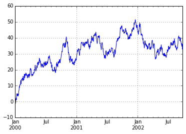
# time series plot
ts = pd.Series(np.random.randn(1000), index=pd.date_range('1/1/2000', periods=1000))
ts = ts.cumsum()
ts.plot()
Out:
<matplotlib.axes._subplots.AxesSubplot at 0xd180438>
In:
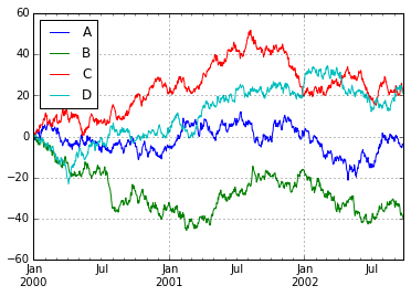
# plot with a data frame
df = pd.DataFrame(np.random.randn(1000, 4), index=ts.index, columns=['A', 'B', 'C', 'D'])
df = df.cumsum()
plt.figure(); df.plot(); plt.legend(loc='best')
Out:
<matplotlib.legend.Legend at 0xd541fd0>
<matplotlib.figure.Figure at 0xd554550>
Input / Output
In:
# write to a csv file
df.to_csv('foo.csv', index=False)

# read file back in
path = r'C:UsersJohnDocumentsIPython Notebooksfoo.csv'
newDf = pd.read_csv(path)
newDf.head()
Out:
| A | B | C | D | |
|---|---|---|---|---|
| 0 | -0.914956 | 0.294759 | 0.143332 | 0.174706 |
| 1 | -0.297442 | 1.640208 | 0.425301 | -0.075666 |
| 2 | -0.762292 | 0.741179 | 0.505002 | -0.128560 |
| 3 | -1.577471 | -0.495294 | 1.803332 | 0.188178 |
| 4 | -0.137486 | -0.676985 | 1.435308 | 0.181047 |
In:
# remove the file
import os
os.remove(path)

# can also do Excel
df.to_excel('foo.xlsx', sheet_name='Sheet1')

newDf2 = pd.read_excel('foo.xlsx', 'Sheet1', index_col=None, na_values=['NA'])
newDf2.head()
Out:
| A | B | C | D | |
|---|---|---|---|---|
| 2000-01-01 | -0.914956 | 0.294759 | 0.143332 | 0.174706 |
| 2000-01-02 | -0.297442 | 1.640208 | 0.425301 | -0.075666 |
| 2000-01-03 | -0.762292 | 0.741179 | 0.505002 | -0.128560 |
| 2000-01-04 | -1.577471 | -0.495294 | 1.803332 | 0.188178 |
| 2000-01-05 | -0.137486 | -0.676985 | 1.435308 | 0.181047 |


近期评论