
Today we will use R to establish a linear relationship between the price of a car and mpg(mileage).
Know about data
First of all, we import the auto.dta and view the first six observations for checking.
library(haven)
auto <- read_dta("auto.dta")
head(auto)
## # A tibble: 6 x 12
##   make  price   mpg rep78 headroom trunk weight length  turn displacement
##   <chr> <dbl> <dbl> <dbl>    <dbl> <dbl>  <dbl>  <dbl> <dbl>        <dbl>
## 1 AMC ~  4099    22     3      2.5    11   2930    186    40          121
## 2 AMC ~  4749    17     3      3      11   3350    173    40          258
## 3 AMC ~  3799    22    NA      3      12   2640    168    35          121
## 4 Buic~  4816    20     3      4.5    16   3250    196    40          196
## 5 Buic~  7827    15     4      4      20   4080    222    43          350
## 6 Buic~  5788    18     3      4      21   3670    218    43          231
## # ... with 2 more variables: gear_ratio <dbl>, foreign <dbl+lbl>
Relationship Between Price and Mpg
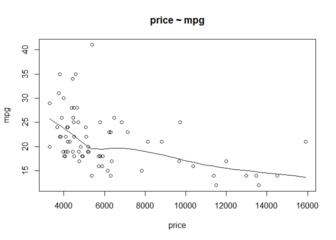
We caculate the correlation between price and mpg. Futhermore, we can draw a scatter plot to sketch their relationship.
cor(auto$price, auto$mpg)
## [1] -0.4685967
scatter.smooth(x=auto$price, y=auto$mpg, main="price ~ mpg",xlab="price",
     ylab="mpg")
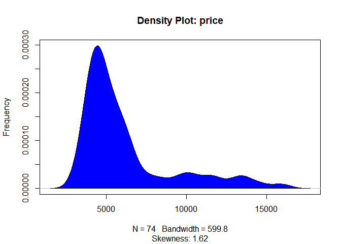
Draw a density plot to scan the distribution of price.
library(e1071)
plot(density(auto$price), main="Density Plot: price", ylab="Frequency", sub=paste("Skewness:", round(e1071::skewness(auto$price), 2)))
polygon(density(auto$price), col="blue")
Linear Regression
Now we find that price and mpg have negative relationship, when mpg increases, price decreases. In order to know it deeply, we use linear regression to analyze.
linearMod <- lm(price ~ mpg, data=auto)
summary(linearMod)
##
## Call:
## lm(formula = price ~ mpg, data = auto)
##
## Residuals:
##     Min      1Q  Median      3Q     Max
## -3184.2 -1886.9  -959.8  1359.7  9669.7
##
## Coefficients:
##             Estimate Std. Error t value Pr(>|t|)
## (Intercept) 11253.06    1170.81   9.611 1.53e-14 ***
## mpg          -238.89      53.08  -4.501 2.55e-05 ***
## ---
## Signif. codes:  0 '***' 0.001 '**' 0.01 '*' 0.05 '.' 0.1 ' ' 1
##
## Residual standard error: 2624 on 72 degrees of freedom
## Multiple R-squared:  0.2196,	Adjusted R-squared:  0.2087
## F-statistic: 20.26 on 1 and 72 DF,  p-value: 2.546e-05
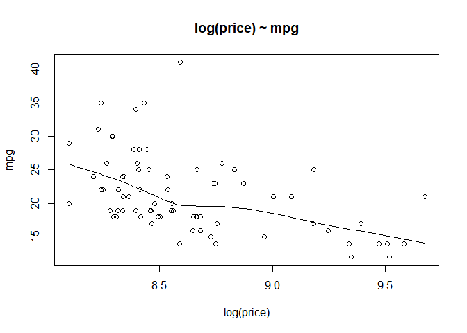
We use log(price) to replace price and do the previous process again.
auto$lp<-log(auto$price)
scatter.smooth(x=auto$lp, y=auto$mpg, main="log(price) ~ mpg",
     xlab="log(price)", ylab="mpg")
linearMod <- lm(lp ~ mpg, data=auto)
summary(linearMod)
##
## Call:
## lm(formula = lp ~ mpg, data = auto)
##
## Residuals:
##      Min       1Q   Median       3Q      Max
## -0.58486 -0.25525 -0.08595  0.22935  1.02393
##
## Coefficients:
##              Estimate Std. Error t value Pr(>|t|)
## (Intercept)  9.349342   0.153489  60.912  < 2e-16 ***
## mpg         -0.033277   0.006958  -4.782 8.93e-06 ***
## ---
## Signif. codes:  0 '***' 0.001 '**' 0.01 '*' 0.05 '.' 0.1 ' ' 1
##
## Residual standard error: 0.344 on 72 degrees of freedom
## Multiple R-squared:  0.2411,	Adjusted R-squared:  0.2305
## F-statistic: 22.87 on 1 and 72 DF,  p-value: 8.93e-06
Conclusion
As seen in the results above, we can find that the p-values and t Statistic are statisticaly significant. But simple linear regression isn’t enough for idenifying casual effect, we will discuss it next time.
Reference
- r-statistics.co by Selva Prabhakaran


近期评论