estimating probabilities

1. Definition of MLE and MAP
2. An example of coin flips
3. Inference
4. More about MAP and MLE
5. Reference

Estimating probabilities is important in statistical research. Today we will talk about two most common approaches to estimate probabilities: maximum likelihood estimation (MLE) and maximum a posteriori estimation (MAP).

Definition of MLE and MAP

• Maximum likelihood estimation (MLE)’s principle is that if we observe training data $D$, we should choose the value of $theta$ that makes $D$ most probable.

$$hat{theta}^{MLE} = argmax_theta{P(D|theta)}$$

• Maximium a posteriori probability (MAP) estimation is to choose the most probable value of $theta$, given the observed training data plus a prior probability distribution $P(theta)$ which captures prior knowledge or assumptions about the value of $theta$.

$$hat{theta}^{MAP} = argmax_theta{P(theta|D)}$$

An example of coin flips

Imagine we flip coins many times, let $X = 1$ if it turns up heads and $X=0$ if it turns up tails. We should estimate the probability that it will turn up heads, that is, to estimate $P(X = 1)$.

We flip the coin n times and observe that it turns up heads $alpha_0$ times, and tails $alpha_1$ times. $n =alpha_0 + alpha_1$.

There are two assumptions:

1. The outcomes of the flips are independent. That means the result of one coin flip has no influence on other coin flips.

2. The outcomes are identically distributed. That means each coin flip has the same value of $theta$.

Inference

The maximum likelihood (MLE) principle involves choosing $theta$ to maximize $P(D|theta)$. We can write formula as follow:

$$P(D=langle{alpha_1,alpha_0}rangle|theta) = theta^{alpha_1}(1-theta)^{alpha_0}$$

This likelihood function is often written $L(theta) = P(D|theta)$. Notice that maximizing $P(D|theta)$ with respect to $theta$ is equivalent to maximizing its logarithm, $ln P(D|theta) $ with respect to $theta$, because $ln x$ increases monotonically with $x$. So we write $l(theta) = ln P(D|theta)$ and find $theta$ which maxmizes $l(theta)$.

$$% <![CDATA[ begin{equation} begin{split} frac{partial{l(theta)}}{partial{theta}} &= frac{partialln{P(D|theta)}}{partial{theta}} \ &= frac{partialln{[theta^{alpha_1}(1-theta)^{alpha_0}]}}{partial{theta}} \ &= frac{partial[alpha_1ln{theta}+alpha_0ln(1-theta)]}{partial{theta}} \ &= alpha_1frac{partiallntheta}{partialtheta} + alpha_0frac{partialln(1-theta)}{partialtheta} \ &= alpha_1frac{1}{theta} - alpha_0frac{1}{1-theta} end{split} end{equation} %]]>$$

We let it equals to zero and simplify it. We can get:

$$hat{theta} = frac{alpha_1}{alpha_1+alpha_0}$$

Also, given observed training data producing $alpha_1$ observed “heads”, and $alpha_2$ observed ”tails”, plus prior information expressed by introducing imaginary “heads” and imaginary “tails”, output the estimate:

$$hat{theta} = frac{alpha_1+gamma_1}{(alpha_1+gamma_1)+(alpha_0+gamma_0)}$$

More about MAP and MLE

What we should know is that MAP needs background assumptions of its value which MLE doesn’t need. In other words, MAP assumes background knowledge is available.

If MAP priors are correct, then MAP is a better estimation than MLE. But if MAP priors are incorrect, MLE is better.

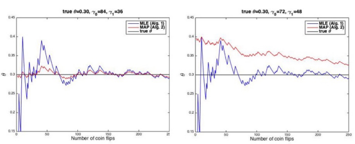
Follow pictures assume $theta = 0.3$ and picture 1 has correct MAP priors but picture doesn’t, the blue line if estimation of MLE and the red line is estimation of MAP. We can discover that MAP is closer to real $theta$ when MAP has correct priors. On the contrary, MLE is closer to real $theta$ when MAP priors are wrong. Also, as the size of the data grows, the MLE and MAP estimates converge toward each other, and toward the correct estimate for $theta$.

Reference

1. Mitchell, ESTIMATING PROBABILITIES: MLE AND MAP