
Theory
The part is an excerpt from Peter Shearer’s SCEC-ERI Back-projection Material
Consider a linea set of equations relating observed data to a model:
using the conventional notation of $d$ for the data vector, $m$ for the model vector, and $G$ for the linear operator that predicts the data from the model. Our goal in geophysical inverse problems is to estimate $m$ from the observations, $d$. Assuming there are more data points than model points, the standard way to solve this problem is to define a residual vector, $r = d - Gm$ , and find the $m$ that minimizes $r · r$. This is the least squares solutions and it can be shown that
However often $G^T G$ is singular or ill-conditioned, or it may simply be too large to invert. What can be done is these cases? The simplest and crudest way to proceed is to make the approximation
in which case we can estimate the model as
The transposed matrix $G^T$ is the adjoint or back-projection operator. Each model point is constructed as the weighted sum of the data points that it affects. Can such a crude approximation be of any use? It’s certainly easy to think of examples $(G^T G) ^{-1} ≈ I$ is completely invalid. However, in real geophysical problems, it’s surprising how often this method works, particularly if a scaling factor is allowed to bring the data and model-predicted data into a better agreement (i.e., assuming $(G^T G) ^{−1} ≈ λI$, where $λ$ is a constant). Indeed, it is sometimes observed that the adjoint works better than the formal inverse because it is more tolerant of imperfections in the data. Jon Claerbout discusses this in a wonderful set of notes (e.g., http://sepwww.stanford.edu/sep/prof/gee/ajt/paper_html/node1.html).
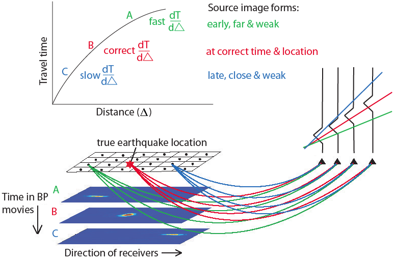
In seismology, our data are typically a set of seismograms. In source inversions, we normally assume that the Earth’s velocity structure is known and we solve for the locations and times of seismic wave radiators (e.g., solving for a slip model). In reflection seismology, we normally assume that the location and time of the source is known and we solve for the location of the reflector(s) that cause the observed arrivals. In each case, the model estimate at each model point is obtained by finding the times in the seismograms at which changes in the model will affect the seismogram. The model estimate from back-projection is obtained by simply summing or stacking the seismogram values at these points. The main thing to compute is the travel time between the model points and each recording station. These give the time shifts necessary to find the times in each seismogram that are sensitive to the model perturbations.
One way of thinking about this is that we have the computer perform a series of hypothesis tests over a time-space model grid. Is there a seismic radiator at this space-time point? If there is, we would expect it to show up in seismograms at these times. If we sum over the seismogram values at these times, we should get a large amplitude. Of course, it is possible that inference from radiation at other model points will cause us to have a biased estimate. But on average, we hope (expect) these other contributions to cancel out. This is the forward-time way of thinking about the problem.
But we could also think about this in reverse time. In this case, we start with the seismograms and project their values backward in time through the model grid. As we do this, we accumulate the values in the model grid points. The model points that are likely sources will experience constructive interference as the time-reversed wavefields focus on these points. This is why this process is sometimes called back-projection or reverse time migration. But the result is exactly the same as the forward modeling approach described in the previous paragraph.
From IRIS
Left unstated in this discussion is how the amplitudes in the seismograms should be scaled. If one wants to recover true model amplitudes, then geometrical spreading and other factors should be taken into account. Often, however, the goal is simply an image of the model and the absolute amplitude is not that important. For example, in reflection seismology, automatic gain control is often used to equalize the contributions from different records and true amplitude information is lost. These amplitude normalization methods can make back-projection more robust with respect to noisy data or uncertainties in the velocity model.
Advantages and disadvantages
These are meant to be a standardized blunt tool to image the time and space history of high-frequency P-waves from large earthquakes. Sometimes, overall rupture features (duration, directivity, length) can be inferred for larger, M > ~7.5, events when two or more arrays are in general agreement with respect to the time and location of bursts of energy. For smaller events, M < ~7.0, rupture characteristics are seldom reliable due to short rupture lengths, however, distinguishing between a simple rupture and an earthquake doublet is sometimes noticeable. These can also show the absolute location of smaller, more point-source like, earthquakes as imaged by the particular receiving array within the 1D reference model.
Artifacts abound and a growing number of fancier approaches and higher resolution results using careful manual processing are appearing in the literature. Caution should be taken to not over-interpret secondary features or a single array’s results for a given earthquake. Forward modeling with synthetic seismograms computed from finite-fault models shows that for some source-receiver array geometries strong artifacts suggesting rupture complexity can sometimes be reproduced from relatively simple models. Finally, these results are fully automated and similar approaches in the research literature will often contain ‘better’ results due to more advanced methods and manual attention to data quality and processing results. Bad back-projections are often the result of bad data selection. Caveat emptor.


近期评论