首页 > itarticle > fast fourier transform

fast fourier transform

admin 11月 13, 2020 0

Theory and Code of FFT

FFT(Fast Fourier transform) is first developed to speed the DFT(Discrete Fourier transform). Below is my matlab code. To be brief, it is similar to an divide and conquer algorithm. The complexity of FFT is O(NlogN).

function [ X ] = ( x, N )
   wn = exp(i*2*pi/N);
   X = 0:N-1;
   if(N==1)
       X(1)=x(1);
       return ;
   end
   y0 = 0:N/2-1; y1 = 0:N/2-1;
   for k = 0:N/2-1
       y0(k+1) = x(k+1) + x(k+1+N/2);
       y1(k+1) = (x(k+1) - x(k+1+N/2))*wn^(k);
   end
   Y0 = FFT(y0, N/2); Y1 = FFT(y1, N/2);
   for k = 0:N/2-1
       X(2*k+1) = Y0(k+1);
       X(2*k+1+1) = Y1(k+1);
   end
end

Usually, the FFT is applied to image processing, where 2-dimensional FFT is used more frequently. Here is the 2-dimensional FFT code.

function [ img ] = FFT2( img, M, N )
   for i = 1:M
       img(i,:) = FFT(img(i,:), N);
   end
   for j = 1:N
       img(:,j) = FFT(img(:,j),M);
   end
end
``` 

After operations in frequency domain, transformation from frequency domain to time domain is necessary. This is often realized by Inverse Fast Fourier transformation(IFFT). The difference between FFT and IFFT
is just the choice of base function in frequency domain. Below is the  and 2-dimensional  code.
```Matlab
function [ X ] = IFFT( x, N )
   wn = exp(-i*2*pi/N);
   X = 0:N-1;
   if(N==1)
       X(1)=x(1);
       return ;
   end
   y0 = 0:N/2-1; y1 = 0:N/2-1;
   for k = 0:N/2-1
       y0(k+1) = x(k+1) + x(k+1+N/2);
       y1(k+1) = (x(k+1) - x(k+1+N/2))*wn^(k);
   end
   Y0 = IFFT(y0, N/2); Y1 = IFFT(y1, N/2);
   for k = 0:N/2-1
       X(2*k+1) = Y0(k+1);
       X(2*k+1+1) = Y1(k+1);
   end
end

function [ img ] = IFFT2( img, M, N )
   for i = 1:M
       img(i,:) = IFFT(img(i,:), N);
   end
   for j = 1:N
       img(:,j) = IFFT(img(:,j),M);
   end
end

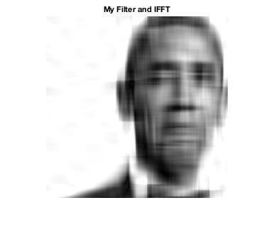
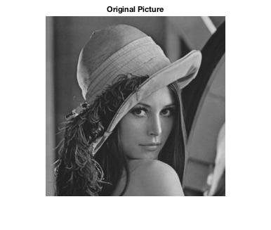
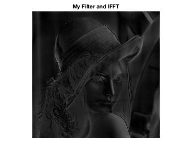
Application of FFT in Imageprocessing

Below is the code I’ve written to do imageprocessing and test my FFT.


clear; clc; close all;
img = imread('aobama.png');
img = rgb2gray(img);
img = im2double(img);
I = imresize(img, [256, 256]);
figure;
imshow(I); title('Original Picture');
%% My FFT2
figure;
imshow(log(abs(fftshift(FFT2(I,256,256)))+1)); title('My FFT');
%% My IFFT2
figure; title('My IFFT');
FFT_I = FFT2(I,256,256)/256.0/256.0;
%FFT_I(1:120,1:120) = 0; FFT_I(256-120+1:256,256-120+1:256:256) = 0; %high pass
FFT_I(5:256-5,5:256-5) = 0; %low pass
imshow(abs(IFFT2(FFT_I,256,256)));title('My Filter and IFFT');

After low pass, the average color of the image is kept but the details become unclear due to loss of high frequency informatino.

After high pass, the details of the image such as edges become clear but the average color changes obviously.