
ABSTRACT
We extend current models to deal with two key challenges present in this task: corpora and vocabulary sizes, and complex, long term structure of language. We perform an exhaustive study on techniques such as character Convolutional Neural Networks or Long-Short Term Memory, on the One Billion Word Benchmark.
Introduction
Models which can accurately place distributions over sentences not only encode complexities of language such as grammatical structure, but also distill a fair amount of information about the knowledge that a corpora may contain.(提取大量关于语料库可能包含的知识的信息).
Language Modeling can apply in speech recoginition, machine translation, text summarization etc. (such as word error rate for speech recognition, or BLEU score for translation).
When trained on vast amounts of data, language models compactly extract knowledge encoded in the training data. For example, when trained on movie subtitles, language models are able to generate basic answers to questions about object colors, facts about people, etc.
language model such as N-grams, only use a short history of previous words to predict the next word, , they are still a key component to high quality, low perplexity Language Modeling. RNNs based language model are great in combination with N-grams.
The contributions:
Unify some of the current research on larger scale LM
Designed a Softmax loss which is based on character level CNNs instead of a full softmax
Reduce the number of parameters
Related Work
Language Models
Much work has been done on both parametric (e.g., log-linear models) and non-parametric approaches (e.g., count-based LMs).
Count-based approaches(based on statistics of N-grams). For example: unigram, bigram, trigram, 5-gram models. Log-linear approaches(based on recurrent neural network). For example: RNN-based, LSTM, GRU.
Convolution Embedding Models
There is an increased interest in incorporating character-level inputs to build word embeddings for various NLP problems, including part-of-speech tagging, parsing and language modeling.
Several approach building word embedding:
Bidirectional LSTMs over the characters.
The recurrent networks process sequences of characters from both sides and their final state vectors are concatenated.
The words characters are processed by a 1-d CNN with max-pooling across the sequence for each convolutional feature. The resulting features are fed to a 2-layer highway network, which allows the embedding to learn semantic representations.
Softmax Over Large Vocabularies
Assigning probability distributions over large vocabularies is computationally challenging. For modeling language, maximizing log-likelihood of a given word sequence leads to optimizing cross entropy between the target probability distribution, and our model predictions $p$. Generaly, predictions come from a linear layer follows by a Sofemax non-linearity: $p(w)={exp(z_w) over sum_{w’ in V} exp(z_{w’})}$,where $z_w$ is the logit corresponding to a word $w$. The logit is generally computed as an inner product $z_w = h^Te_w$ where $h$ is a context vector and $e_w$ is a “word embedding” for $w$.
The main challenge when $|V|$ is very large is the fact that computing all inner products between h and all embeddings becomes prohibitively slow during training. Several approaches have been proposed to cope with the scaling issue: importance sampling , Noise Contrastive Estimation (NCE), self normalizing partition functions, Hierarchical Softmax.
Language Modeling Improvements
Recurrent Neural Networks based LMs employ the chain rule to model joint probabilities over word sequences:
where the context of all previous words is encoded with an LSTM, and the probability over words uses a Softmax.
Relationship between Noise Contrastive Estimation and Importance Sampling
A large scale Softmax is necessary for training good LMs because of the vocabulary size. A Hierarchical Softmax employs a tree in which the probability distribution over words is decomposed into a product of two probabilities for each word, greatly reducing training and inference time as only the path specified by the hierarchy needs to be computed and updated. Choosing a good hierarchy is important for obtaining good results and we did not explore this approach further for this paper as sampling methods worked well for our setup.
Sampling approaches are only useful during training, as they propose an approximation to the loss which is cheap to compute (also in a distributed setting) – however, at inference time one still has to compute the normalization term over all words. Noise Contrastive Estimation (NCE) pro-
poses to consider a surrogate binary classification task in which a classifier is trained to discriminate between true data, or samples coming from some arbitrary distribution. If both the noise and data distributions were known, the optimal classifier would be:
where $Y$ is the binary random variable indicating whether w comes from the true data distribution, $k$ is the number of negative samples per positive word, and $p_d$ and $p_n$ are the data and noise distribution respectively (we dropped any dependency on previous words for notational simplicity). It is easy to show that if we train a logistic classifier $p_{theta}(Y=true|w) = sigma(s_{theta}(w,h)-logkp_n(w))$, then, $p’(w)=softmax(s_{theta}(w,h))$ is good approximation of $p_d(w)$($s_{theta}$ is a logit which e.g. an LSTM LM computes).
The other technique, which is based on importance sampling (IS), proposes to directly approximate the partition function (which comprises a sum over all words) with an estimate of it through importance sampling. Though the methods look superficially similar, we will derive a similar surrogate classification task akin to NCE which arrives at IS, showing a strong connection between the two.
Suppose that, instead of having a binary task to decide if a word comes from the data or from the noise distribution, we want to identify the words coming from the true data distribution in a set
$W={w_1,…,W_{k+1}}$, comprised of $k$ noise samples and one data distribution sample. we can train a multiclass loss over a multinomial random variable $Y$ which maximizes $logp(Y=1|W)$, assuming w.l.o.g. that $w_1 in W$ is always the word coming from true data. By Bayes rule, and ignoring terms that are constant with respect to $Y$, we can write:
and, following a similar argument than for NCE, if we define :$p(Y=k|W) = softmax(s_{theta}(w_k)-logp_n(w_k))$ then $p’(w)=softmax(s_{theta}(w,h))$. Note that the only difference between NCE and IS is that, in NCE, we define a binary classification task
between true or noise words with a logistic loss, whereas in IS we define a multiclass classification problem with a Softmax and cross entropy loss. We hope that our derivation helps clarify the similarities and differences between the two. In particular, we observe that IS, as it optimizes
a multiclass classification task (in contrast to solving a binary task), may be a better choice. Indeed, the updates to the logits with IS are tied whereas in NCE they are independent.
CNN softmax
The character-level features allow for a smoother and compact parametrization of the word embeddings. Recall that the Softmax computers a logit as $z_w=h^Te_w$ where $h$ is a context vector and $e_w$ is a “word embedding” for $w$. Instead of building a matrix of$|V| times |h|$(whose rows correspond to $e_w$), we produce $e_w$w with a CNN over the characters of $w$ as$e_w=CNN(chars_w)$– we call this a CNN Softmax. We used the same network architecture to dynamically generate the Softmax word embeddings without sharing the parameters with the input word-embedding sub-network. For inference, the vectors $e_w$ can be precomputed, so there is no computational complexity increase w.r.t. the regular Softmax.
When using an importance sampling loss only a few logits have non-zero gradient (those corresponding to the true and sampled words). With a Softmax where $e_w$ are independently
learned word embeddings, this is not a problem. But we observed that, when using a CNN, all the logits become tied as the function mapping from $w$ to $e_w$ w is quite smooth. As a result, a much smaller learning rate had to be used. Even with this, the model lacks capacity to differentiate
between words that have very different meanings but that are spelled similarly. Thus, a reasonable compromise was to add a small correction factor which is learned per word,
such that:
where M is a matrix projecting a low-dimensional embedding vector $corr_w$ back up to the dimensionality of the projected LSTM hidden state of h. This amounts to adding a bottleneck linear layer, and brings the CNN Softmax much closer to our best result, where adding a 128-dim correction halves the gap between regular and the CNN Softmax.
Aside from a big reduction in the number of parameters and incorporating morphological knowledge from words, the other benefit of this approach is that out-of-vocabulary (OOV) words can easily be scored. This may be useful for other problems such as Machine Translation where handling out-of-vocabulary words is very important . This approach also allows parallel training
over various data sets since the model is no longer explicitly parametrized by the vocabulary size – or the language.
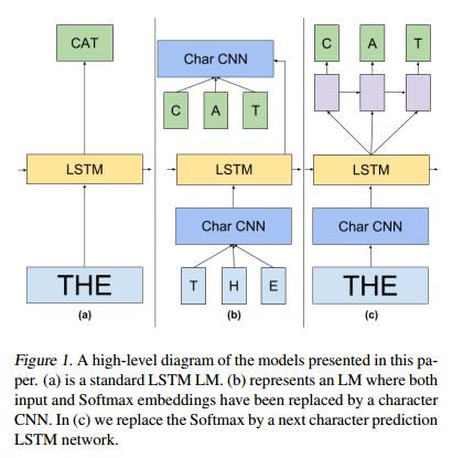
Char LSTM Predictions
The CNN Softmax layer can handle arbitrary words and is much more efficient in terms of number of parameters than the full Softmax matrix. It is, though, still considerably slow, as to evaluate perplexities we need to compute the partition function. A class of models that solve this prob-
lem more efficiently are character-level LSTMs. They make predictions one character at a time, thus allowing to compute probabilities over a much smaller vocabulary. On the other hand,
these models are more difficult to train and seem to perform worse even in small tasks like PTB Most likely this is due to the sequences becoming much longer on average as the LSTM reads the input character by character instead of word by word.
Thus, we combine the word and character-level models by feeding a word-level LSTM hidden state h into a small LSTM that predicts the target word one character at a time. In order to make the whole process reasonably efficient, we train the standard LSTM model until convergence, freeze its weights, and replace the standard word-level Softmax layer with the aforementioned character-level LSTM.


近期评论