reading note: $s^3fd$: single shot scale

TITLE: $S^3FD$: Single Shot Scale-invariant Face Detector

AUTHOR: Shifeng Zhang, Xiangyu Zhu, Zhen Lei, Hailin Shi, Xiaobo Wang, Stan Z. Li

ASSOCIATION: Chinese Academy of Sciences

FROM: arXiv:1708.05237

CONTRIBUTION

1. Proposing a scale-equitable face detection framework with a wide range of anchor-associated layers and a series of reasonable anchor scales so as to handle dif- ferent scales of faces well.
2. Presenting a scale compensation anchor matching strategy to improve the recall rate of small faces.
3. Introducing a max-out background label to reduce the high false positive rate of small faces.
4. Achieving state-of-the-art results on AFW, PASCAL face, FDDB and WIDER FACE with real-time speed.

METHOD

There are mainly three reasons that why the performance of anchor-based detetors drop dramatically as the objects becoming smaller:

1. Biased Framework. Firstly, the stride size of the lowest anchor-associated layer is too large, thus few features are reliable for small faces. Secondly, anchor scale mismatches receptive field and both are too large to fit small faces.
2. Anchor Matching Strategy. Anchor scales are discrete but face scale is continuous. Those faces whose scale distribute away from anchor scales can not match enough anchors, such as tiny and outer face.
3. Background from Small Anchors. Small anchors lead to sharp increase in the number of negative anchors on the background, bringing about many false positive faces.

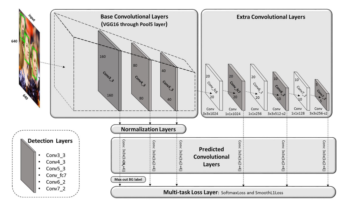
The architecture of Single Shot Scale-invariant Face Detector is shown in the following figure.

Scale-equitable framework

Constructing Architecture

• Base Convolutional Layers: layers of VGG16 from conv1_1 to pool5 are kept.
• Extra Convolutional Layers: fc6 and fc7 of VGG16 are converted to convolutional layers. Then extra convolutional layers are added, which is similar to SSD.
• Detection Convolutional Layers: conv3_3, conv4_3, conv5_3, conv_fc7, conv6_2 and conv7_2 are selected as the detection layers.
• Normalization Layers: L2 normalization is applied to conv3_3, conv4_3 and conv5_3 to rescale their norm to 10, 8 and 5 respectively. The scales are then learned during the back propagation.
• Predicted Convolutional Layers: For each anchor, 4 offsets relative to its coordinates and $N_{s}$ scores for classification, where $N_s=N_m+1$ ($N_m$ is the maxout background label) for conv3_3 detection layer and $N_s=2$ for other detection layers.
• Multi-task Loss Layer: Softmax loss for classification and smooth L1 loss for regression.

Designing scales for anchors

• Effective receptive field: the anchor should be significantly smaller than theoretical receptive field in order to match the effective receptive field.
• Equal-proportion interval principle: the scales of the anchors are 4 times its interval, which guarantees that different scales of anchor have the same density on the image, so that various scales face can approximately match the same number of anchors.

Scale compensaton anchor matching strategy

To solve the problems that 1) the average number of matched anchors is about 3 which is not enough to recall faces with high scores; 2) the number of matched anchors is highly related to the anchor scales, a scale compensation anchor matching strategy is proposed. There are two stages:

• Stage One: decrease threshold from 0.5 to 0.35 in order to increase the average number of matched anchors.
• Stage Two: firstly pick out anchors whose jaccard overlap with tiny or outer faces are higher than 0.1, then sorting them to select top-N as matched anchors. N is set as the average number from stage one.

Max-out background label

For conv3_3 detection layer, a max-out background label is applied. For each of the smallest anchors, $N_m$ scores are predicted for background label and then choose the highest as its final score.

Training

1. Training dataset and data augmentation, including color distort, random crop and horizontal flip.
2. Loss function is a multi-task loss defined in RPN.
3. Hard negative mining.

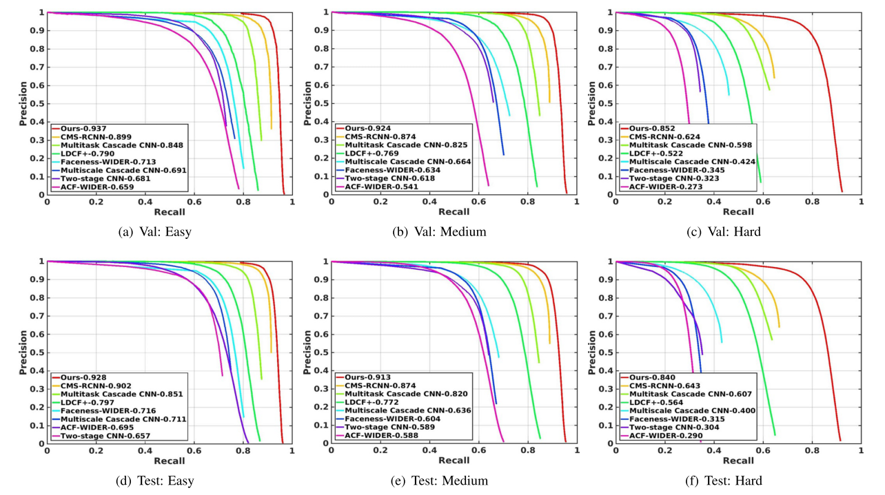
The experiment result on WIDER FACE is illustrated in the following figure.