matrix factorization for recommender systems

Matching users with most appropriate items is the key the enhancing user satisfaction and loyalty. That’s why recommender systems are so important for companies involve specific business.

Matrix factorization models perform much better to classic Nearst-Neighbor models (at least in Netflix Prize competition), which allow incorporation of additional info such as implicit feedback, temporal effect and confidence levels.

Basically recommender systems are based on two strategies:

• Content Filtering

Content based recommendations create user profile and item profile for users and items, broadly speaking it could be vector representation, e.g. item (movies) could use genre / actors / popularity; user could use demographic / preferences. To make recommendations, user profile need to associate with product to get matched. It requires external data which might need heavy domain knowledge and not easy to collect.

• Collaborative Filtering

Collaborative filtering is based on historical data about interactions between user and item, such as user ratings on items. Therefore no domain knowledge needed - which could be a issue for content based recommendation since different business direction could have huge difference. But it could suffer from cold start, which means not enough historical data at early stage for the system or introduction of new users and new items.

There are two types of model for collaborative filtering:

1. nearest-neighbor models: include user-based and item-based collaborative filtering;
2. latent factor models: try to explain the ratings by characterizing both user and items on, the factors could be either interpretable or uninterpretable; a user’s predicted ratings for item relate to the dot product of user-factor and item-factor.

Recommender systems rely on different types of input data which are often placed in matrices with one dimension represents users and another dimension represents items, the most convenient data is explicit data which includes the explicit input by users regarding their interests in items, such as ratings. However this matrix is usually sparse since many users won’t rate on too many items.

Some of the most successful latent factor models are based on matrix factorization. One of the advantages of matrix factorization is that it allows incorporates additional information. When explicit data is not available, the recommender system can infer user preferences using implicit feedback, such as: purchase history, browsing history, search patterns, actions when browsing (mouse movements). Implicit feedback usually could be denoted by binary representations, so it is typically represented as dense matrix.

Matrix factorization models map both users and items to a joint latent factor space of dimensionality (f), such that user-item interactions are modeled as inner products in this space. Each user (u) is associated with a vector (p_{u}in R^{f}), each item (i) is associated with a vector (q_{i}in R^{f}). For a given user (u) the elements of (p_{u}) measures the extent of interest of user has, in items that are high on corresponding factors. The dot product (q_{i}^{top}p_{u}) captures the interactions between user and item, this is actually an approximation:

[
hat{r}_{ui} = q_{i}^{top}p_{u}.
]

SVD could be used to get user and item vectors. However, classical SVD might not work directly on rating matrix since it’s sparse and incomplete, and it’s highly prone to overgitting.

One of the solutions is imputation, but this could be very expensive and introduce bias. More recent works suggested directly model on non-missing data, from optimization perspective, user and item vectors could be learned by

[
min_{q, p} sum_{(u,i)in k} left(r_{ui} -q_{i}^{top}p_{u} right)^2 + lambdaleft(||q_{i}||_{2}^{2} + ||p_{u}||_{2}^{2}right),
]

where (k) is the set of user-item pairs observed.

There are 2 approaches proposed to solve the above optimization problem: SGD and Alternating least squares. ALS is preferred in two cases:

1. system can be parallelized;
2. system incorporates implicit feedbacks (dense matrix).

Ratings by different users on different items could have biases, independent of any interactions. For example, some users give higher ratings, some items receives higher ratings. Therefore, the system tries to identify the portion of these values that individual user or item biases can explain, subjecting only the true interaction portion of the data to factor modeling. A first-order approximation for bias is as follows:

[
b_{ui} = mu + b_{u}+ b_{i},
]

where (mu) is the overall average rating, (b_{u}) and (b_{i}) denote for the item and user observed deviations from average. The adjusted predicted rating is
[
hat{r}_{ui} = b_{ui} + q_{i}^{top}p_{u} = mu + b_{u} + b_{i} + q_{i}^{top}p_{u}.
]

and learning problem is adjusted as

[
min_{q, p, b} sum_{(u,i)in k} left(r_{ui} -mu - b_{u} - b_{i} - q_{i}^{top}p_{u} right)^2 + lambdaleft(||q_{i}||_{2}^{2} + ||p_{u}||_{2}^{2} + b_{u}^{2} + b_{i}^{2}right).
]

Add implicit data is one way to tackle cold start problem. Considering binary representations, (N(u)) denotes the set of items (a neighbor of items) for user (u) expressed an implicit preference (such as viewed, cliked), item are assocated with (x_{i}in R^{f}). Accordingly, a user who showed a preference for items in (N(u)) is characterized by

[
sum_{iin N(u)} x_{i}, text{ or } |N(u)|^{1/2}sum_{iin N(u)}x_{i}^{9/2} text{ (normalized)}
]

Another implicit source is from users, each user attribute (such as demographic info: gender, age) is denoted by (A(u)), and sum of factor vector (y_{a}in R^{f}) corresponds to attributes to describe a user:

[
sum_{ain A(u)} y_{a}.
]

Then the predited rating is adjusted as

[
hat{r}_{ui} = mu + b_{u} + b_{i} + q_{i}^{top}left(p_{u} + |N(u)|^{1/2}sum_{iin N(u)}x_{i}^{9/2} + sum_{ain A(u)} y_{a}right).
]

Matrix factorization models also lends itself well to modeling temporal effects which could significantly improve the accuracy. Factorizing ratings into distinct terms allows the system to treat different temporal aspects separately. The biases terms vary over time, the could be re-parameterized with time factor: item biases - (b_{i}(t)); user biases - (b_{u}(t)); user preference - (p_{u}(t)). These changes incorporate the facts that:

• item popularity could change over time
• users’ baseline rating could change over time
• interaction between user and item also could change

Therefore the predicted rating is adjusted as

[
hat{r}_{ui}(t) = mu + b_{u}(t) + b_{i}(t) + q_{i}^{top}p_{u}(t).
]

Sometimes not all observed ratings should be assigned the same weight or confidence. Also, for systems built based on implicit feedback, users’ exact preference level are hard to quantify. Confidence can stem from available data such as how much time the user watched a certain item or how frequently a user bought certain item. The confidence in observing (r_{ui}) is denoted as (c_{ui}), therefore the learning problem is adjusted as

[
min_{q, p, b} sum_{(u,i)in k} c_{ui}left(r_{ui} -mu - b_{u} - b_{i} - q_{i}^{top}p_{u} right)^2 + lambdaleft(||q_{i}||_{2}^{2} + ||p_{u}||_{2}^{2} + b_{u}^{2} + b_{i}^{2}right).
]

The winning solution for Netflix Prize competition consists of more than 100 different predictor sets, the majority of which are matrix factorization models. A comparison of different settings of matrix factorization models is shown as follows

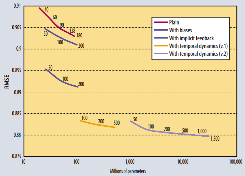
As you can see the temporal components significantly reduce the RMSE.