fourier transformation

The steps for calculate Fourier transform :

1. centralize the original image with f(x,y) ×(-1)^(x+y)
2. Apply Fourier transform to the image
3. get abs(Spectrum) from the image
4. Apply Fourier log transform.
5. Apply scaling.

In fact, I use only one function for DFT and IDF because:

  def dft2d(img, flags):
      if flags == 1:
          return Fdft2d(img)
      elif flags == -1:
          res = np.conjugate(img)
          #return np.conjugate(Fdft2d(img))
          return np.conjugate(Fdft2d(img))

At the first, I treated the 2d Fourier transform using 1d method, which is:

The time complexity of the transform algorithm is O(n^4) which is too slow and I use almost 24 hours to run the program using python. After that I ask a question and I get the answer.

Because the Fourier transform is linear and can divided into two steps for implement. First, calculate Fourier transform for cols and then for the rows. Surprised and luckily, its time complexity is O(n^3) which can be done in few minutes.

The core algorithm is:

    for u in xrange(height):
      for v in xrange(width):
        for y in xrange(width):
            Fourier_img0[u, v] += img[u,y] * (np.exp(-1j*2*np.pi*(float(v*y)/width)))
    for u in xrange(height):
      for v in xrange(width):
        for x in xrange(height):
            Fourier_img[u, v] += Fourier_img0[x, v] * (np.exp(-1j*2*np.pi*(float(u*x)/height)))

Using the two steps to calculate the whole image.

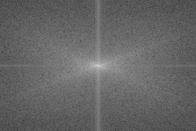
Fourier Spectrum:¶

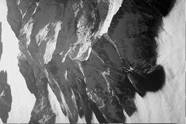
Inverse Fourier Transform¶

Pay attention to the edge of the picture appears a small impurity due to the Transformation error(zero padding)

Fast Fourier Transform¶

First we have the following thinkings:

1. Inverse Fourier Transform is the same as Fourier Transform.
2. The method in 1d Fourier transform can be applied to 2d as well.
3. According to Symmetry, the points in the dialog is at the same value.
4. We have the following equation:

We split a single DFT into two smaller DFT. One odd, one even. So far, we have not save computational overhead, each part contains (n / 2) of N amount of computation, in general, is n.

There is a question “However, your implementation may be limited to images whose sizes are integer powers of 2”, and we can simply padding the image to powers of 2. I have two methods for the users:

1. Padding the image to powers of 2.
2. When the program divide the image into some sub-image that is not powers of 2, DFT_Slow will be applied.

The core algorithm:

1. First we implement 1d fft using the thoughts above.

        def fft(x):
          N = len(x)
          if N <= 1:
            return x
          elif N % 2 != 0:
            return DFT_slow(x)
          else:
            even = fft(x[::2])
            odd = fft(x[1::2])
          return np.concatenate([[even[k] + np.exp(-2j*np.pi*k/N) * odd[k] for k in

2.implentment the 2d fft using 1d fft and using the divide method in fft2d:

def Ffft2d(img):
  height = len(img)
  width = len(img[0])
  Fourier_img0 = np.zeros((height,width),np.complex256)
  for u in xrange(height):
    Fourier_img0[u] = np.array(fft(img[u]))
  Fourier_img = np.zeros((height,width),np.complex256)
  for v in xrange(width):
    Fourier_img[:,v] = fft(Fourier_img0[:,v])
  return Fourier_img

As a result, we get the fft2d. And fft is more fast than dft, we can calculate a image in seconds rather minutes. For example, dft2d use 3~4 minutes to process the image “14.png”, but fft use only some seconds to process.

FFT Fourier Spectrum:¶

IFFT Image:¶

Github¶

https://github.com/ghostbody/Image-Processing