
LinearRegression fits a linear model with coefficients $w = (w_1, …, w_p)$ to minimize the residual sum of squares between the observed responses in the dataset, and the responses predicted by the linear approximation.
Step 0
The parameters t1 t2 are set to 0
Step 1
Calculate the hypothesis for each data point
Step 2
Calculate the cost function
step 3
Calculate the partial derivatives of the cost function with respect to parameters
step 4
Update the parameters
Notation
- x - feature
- y - target values
- m - size of data set
- $alpha$ - learing rate
- $theta_0, theta_1$ - parameters
- $h(x) = theta_0 + theta_1x$ - hypothesis function
- $E(theta_0, theta_1) = frac{1}{2m}sum_{i = 1}^mleft(h_i(x) - y_iright)^2$ - cost function
python sample code
print(__doc__)
import matplotlib.pyplot as plt
import numpy as np
from sklearn import datasets, linear_model
from sklearn.metrics import mean_squared_error, r2_score
# Load the diabetes dataset
diabetes = datasets.load_diabetes()
# Use only one feature
diabetes_X = diabetes.data[:, np.newaxis, 2]
# Split the data into training/testing sets
diabetes_X_train = diabetes_X[:-20]
diabetes_X_test = diabetes_X[-20:]
# Split the targets into training/testing sets
diabetes_y_train = diabetes.target[:-20]
diabetes_y_test = diabetes.target[-20:]
# Create linear regression object
regr = linear_model.LinearRegression()
# Train the model using the training sets
regr.fit(diabetes_X_train, diabetes_y_train)
# Make predictions using the testing set
diabetes_y_pred = regr.predict(diabetes_X_test)
# The coefficients
print('Coefficients: n', regr.coef_)
# The mean squared error
print("Mean squared error: %.2f"
% mean_squared_error(diabetes_y_test, diabetes_y_pred))
# Explained variance score: 1 is perfect prediction
print('Variance score: %.2f' % r2_score(diabetes_y_test, diabetes_y_pred))
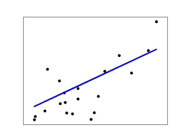
# Plot outputs
plt.scatter(diabetes_X_test, diabetes_y_test, color='black')
plt.plot(diabetes_X_test, diabetes_y_pred, color='blue', linewidth=3)
plt.xticks(())
plt.yticks(())
plt.show()


近期评论